Overview
Mergesort
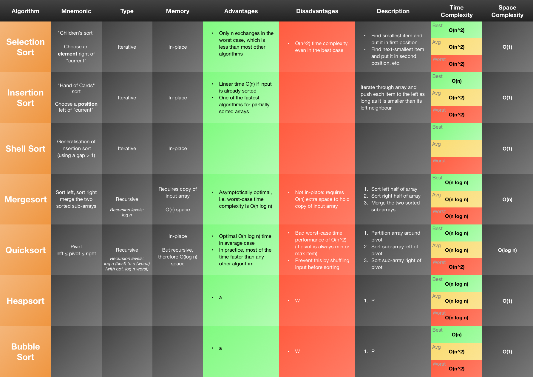
- Asymptotically optimal ($\O(n\,\Log\,n)$) in the worst case
- How to obtain this result is not trivial
- However, not in-place
- Uses $n$ memory for temporary holding the array to sort
- Also $\Log\,n$ recursive call levels, but this is non-dominant compared to $n$
- Thus, space complexity is $\O(n)$
Quicksort
- Asymptotically optimal ($\O(n\,\Log\,n)$) in the average case
- However, ($\O(n^2)$) in the worst case (if always biggest or smallest element is chosen as pivot, e.g. if array is already sorted)
- Counteract by shuffling the array before applying quicksort
- However, ($\O(n^2)$) in the worst case (if always biggest or smallest element is chosen as pivot, e.g. if array is already sorted)
- In-place
- Only algorithm in this list that combines $\O(n\,\Log\,n)$ time complexity and in-place sorting
- However, quicksort is recursive, and there are $\Log\,n$ levels of recursive calls (with some optimisations also in the owrst case)
- Thus, space complexity is $\O(\Log\,n)$
- In practice for most applications faster than any other compare-based sorting algorithm
Selection Sort
In theory: find smallest element and put it in first position, find second-smallest element and put it in second position, etc.
In practice: find the smallest element in the array and swap it with the first element of the array. Then find the smallest element in the remaining part of the array, and swap it with the second element of the array, etc.
for i in (0 to a.end)
    min = index of smallest element of a[i to a.end]
    swap(a[i], a[min])
Performance
- Time: $O(n^2)$
- Memory: in-place
Worst case:
- Number of comparisons: $\frac{n^2}{2}$
- Number of exchanges: $n$
Best case:
- Number of comparisons: $\frac{n^2}{2}$
- Number of exchanges: 0
Special Features
- The initial order of the array has no impact on the number of comparisons (unlike e.g. insertion sort)
- The worst-case number of $n$ exchanges (data moves) is smaller than for most other algorithms.
- Each element is moved in a single move to its final position
Insertion Sort
In theory: for each element, starting with second element from the left, insert it into the correct positions among the elements to its left (the elements to the left of the current element will always be sorted).
In practice: for each element, starting with second element from the left, compare it to the element immediately to its left, and if it’s less than the left-neighbour, swap the two. Repeat this with the new left-neighbour of the element, until encountering a neighbour for which the current element is greater than or equal.
for i in (1 to a.end)
    c = i
    while c > 0 && a[c] < a[c-1]
        swap(a[c], a[c-1])
        c = c - 1
Performance
- Time: $O(n^2)$
- Memory: in-place
Worst case (array sorted in reverse order):
- Number of comparisons: $\frac{n^2}{2}$
- Number of exchanges: $\frac{n^2}{2}$
Average case:
- Number of comparisons: $\frac{n^2}{4}$
- Number of exchanges: $\frac{n^2}{4}$
Best case (array sorted in correct order):
- Number of comparisons: $n-1$
- Number of exchanges: 0
Special Features
- Uses only linear time if the array is already sorted (best case)
- One of the fastest solutions for partially sorted arrays
Insertion Sort vs. Selection Sort
- Selection sort: not touching anything to the left of the current element, looking at everything to the right of the current element.
- Insertion sort: not touching anything to the right of the current element, toucing part of the elements to the left of the current element.
Shellsort
- Named after its inventor Donald Shell
- Generalisation of insertion sort
- Insertion sort is a special case of shell sort where the gap sequence consists of the single value 1
Idea
Insertion sort is slow because the current element is compared each time to its immediate left-neighbour, and then, if it’s smaller, moved one position to the left. Thus, if the current element has to traverse a large portion of the array (e.g. if it’s the smallest element but is at the far right of the array), it takes a large number of steps.
Shellsort addresses this problem by comparing the current element with the element that is $h$ positions to the left. Thus, if the current element has to traverse a large portion of the array, it moves much faster to its appropriate final position.
This process is repeated with decreasing values for $h$, each interation making the array “a bit more sorted”, but probably not yet completely sorted. The last iteration is always with $h=1$, which equals insertion sort, and definitely sorts the array.
The sequence of values used for $h$ is called the gap sequence, and it heavily influences the time performance of the algorithm.
Pseudocode
seq = generate_gap_sequence()  // e.g. (40, 13, 4, 1)
for (h in seq)
    for i in (h to a.end)  // Insertion sort with h substituted for 1
        c = i
        while (c >= h && a[c] < a[c-h])
            swap(a[c], a[c-h])
            c = c - h
Performance
- Time: depends on the gap sequence; in general, with suitable gap sequences, it’s less than quadratic, e.g. $O(n^{\frac{3}{2}})$
- Memory: in-place
Special Features
- One of the few algorithms for which no clear time complexity profile can be given, because the time performance depends on the used gap sequence.
Mergesort
- Linearithmic ($\Theta(n \, \Log \, n)$), but not in-place
- Uses the divide and conquer paradigm of algorithm design
Idea
We can easily merge two sorted arrays by repeatedly taking the smaller element of the two “lower ends” of the sorted input arrays and insert it into the output array. In this way, the output array will also be sorted.
Cut array in half, recursively sort each half, and then merge the sorted halves. The recursive base case is when a sub-array has size 1, in which case it is automatically sorted, and it can be merged with another sorted sub-array.
Pseudcode
sort a
    if (a.size == 1) return           // Recursive base case
    sort(a.left_half)                 // Recursive call
    sort(a.right_half)                // Recursive call
    merge(a.left_half, a.right_half)  // Do work

// The heart of the algorithm (doing the actual work)
merge a1 a2
    for i in (0 .. a.length)
        a[i] = min(a1, a2)
Performance
- Time: $O(n \, \Log \, n)$
- Memory: $O(n)$ (not in-place)
Worst case:
- Number of compares: $n \, \Log \, n$
- Number of array accesses: $6 \cdot n \, \Log \, n$
Best case:
- Number of compares: $\frac{1}{2} \cdot n \, \Log \, n$
Special Features
- Mergesort is an asymptotically optimal compare-based algorithm
- Its worst-case performance is $O(n \, \Log \, n)$, which matches the theoretical worst-case lower bound for compare-based algorithms
Quicksort
- Average-case time performance of $\Theta(n \, \Log \, n)$, and in-place
- Worst-case time performance of $\Theta(n^2)$
- Uses the divide and conquer paradigm, like mergesort
Idea
In theory: pick a random pivot element and rearrange the array so that all elements smaller than the pivot are to the left of it, and all elements greater than the pivot are to the right of it. Now the pivot is in its final position, and the sub-arrays to the left and right of it can be sorted independently from each other by calling quicksort on them recursively.
In practice: pick the last (or first) element of the array as the pivot. Then traverse the array sequentially and maintain three partitions: (1) smaller (or equal) than pivot, (2) greater (or equal) than pivot, (3) uninspected. The “uninspected” partition will be empty when the array is completely traversed. Finally move the pivot element between the “smaller than pivot” and “greater than pivot” partitions, and call quicksort on these two partitions recursively.
Pseudocode
sort a, lo, hi
    if (lo > hi) return           // Recursive base case
    pivot = partition(a, lo, hi)  // Do work
    sort(a, lo, pivot-1)          // Recursive call
    sort(a, pivot+1, hi)          // Recursive call

// The heart of the algorithm (doing the actual work)
partition a, lo, hi
    pivot = hi              // Pick last element of array as pivot
    rightmostLeft = lo - 1  // Rightmost element of "smaller than pivot" partition
    for i in (lo .. hi-1)
        if (a[i] < a[pivot])  // Move element inside "smaller than pivot"  partition
            rightmostLeft++
            swap(a[rightmostLeft], a[i])
    swap(a[rightmostLeft + 1], a[pivot]  // Exchange pivot with leftmost of "greater than pivot" partition
    return rightmostLeft + 1;
Performance
Memory
In-place
Time
Best case (pivot is always median element):
- $O(n \, \Log \, n)$
- Both partitions are of equal size (like in mergesort), which results in a recursion tree of height $\Log \, n$.
** Average case:**
- $O(n \, \Log \, n)$
- Still $O(n \, \Log \, n)$, although with higher contants than the best case.
Worst case (pivot is always smallest or largest element):
This may happen if the array is already sorted.
- $O(n^2)$
- One of the partitions is always empty, the other contains all the elements except the pivot. Thus, the recursion tree has height $n$.
Special Features
- Nearly optimal time performance in the best case, however in the worst case the time performance is not better than selection sort or insertion sort
- To cancel the effect of unsuited input that would provoke the worst case (e.g. if the array is already sorted), the input array can be randomly shuffled before sorting.
Quicksort vs. Mergesort
- Both algorithms are recursive and use the divide and conquer approach
- Mergesort makes the recursive calls first, and only then modifies the array
- That is, it starts modifying the array in the tiny partitions
- Quicksort modifies the array first, and then makes the recursive calls
- That is, it starts modifying the array in the biggest possible partitions
- For mergesort, the number of recursion levels (height of recursion tree) is always $\Log \, n$
- Because all partitions are split in half
- For quicksort, the number of recursion levels is $\Log \, n$ in the best case, and $n$ in the worst case
- Because the relative sizes of the partitions depend on the value of the randomyl chosen pivot element
- Quicksort is generally faster than mergesort in the best case, because its inner loop does fewer data movements
Heapsort
- Can be seen as a more sophisticatd version of selection sort structuring the unsorted item as a max-heap rather than as an unstructured array.